User Guide & Reference

The Systems Thinking Project at the Design & Intelligence Lab at the Georgia Institute of Technology broadly focuses on teaching users at various levels to engage in thinking about complex and, especially, ecological systems. The project specifically addresses multiple specific tasks and abilities:

Helping users understand complex systems through the construction of conceptual models using the Structure-Behavior-Function (SBF) modeling notation models (Goel et al. 2010; Goel et al. 2013).
Providing feedback on model construction through dynamically-generated invokable simulations based on conceptual models (Vattam, Goel, & Rugaber 2010; Joyner, Goel, & Papin 2014).
Facilitating the broader process of scientific inquiry, grounded in model construction (Joyner, Majerich, & Goel 2013).
Providing personalized feedback on modeling and inquiry through context-aware tutoring agents (Joyner & Goel 2014).

The Systems Thinking project has been under active development for over ten years. Over one thousand users have used the tools constructed within the project. The latest tool release in the System Thinking Project is the Virtual Ecological Research Assistant (VERA) which is integrating reference research tools such as the Smithsonian’s Encyclopedia of Life (EOL) and IBM Watson to assist researchers with processing both structured and unstructured information for their model construction. The goal of VERA is to provide non-professionals with the ability to build and simulate conceptual scientific models.

System requirements

While in theory all modern web browsers should interpret Javascript and HTML the same, there are always inconsistencies in the implementations. As such, while VERA was developed using mature open source web libraries and common HTML5 and Javascript code standards, some browsers still perform more reliably than others. The recommended browsers to use with VERA are:

Google Chrome (recommended latest release 68.0.3440.106)
Mozilla Firefox (versions 57+, recommended latest release 61.0.2)

Apple’s Safari and Microsoft’s Edge browsers are not fully supported yet, and their use is discouraged at this time.

Accessing the system

The VERA application is currently hosted at the following URL:

http://vera.cc.gatech.edu

When you visit this site, you should see the following home page:

Click on the Login link in the upper right corner of the page to browse to the login page:

Clicking on Georgia Tech under “SIngle Sign On Options” will redirect you to the Georgia Tech Passport system, where you can log in using your normal GT credentials. After logging in successfully, you will be redirected back to the VERA site displaying your personal dashboard page:

Note that you might not be challenged by GT Passport for a login if you have already been authenticated for another web application. In this case you will simply be redirected to your new user landing page on VERA.

Conceptual modeling of an ecological system

The goal of the VERA tool is to allow a researcher to construct a conceptual model of an ecological system and simulate the system’s behavior. This allows the researcher to gain valuable insight into the ecological system as well as how the different Components in the system interact. The main steps in this process are:

Identify a phenomenon that is to be explored with the model.
Propose a hypothesis to explain the phenomenon.
Create a conceptual model of the ecological system, which will be the base for your experimentation.
Execute simulations of your models, refining the simulation parameters and/or the model in an experimentation feedback loop to test your hypothesis.

1. Identify the phenomenon

The first step in building a conceptual model in VERA is to identify the phenomenon that is to be investigated. A phenomenon is an unusual occurrence/observation that requires explanation. For example:

In a census of marine species, it was observed that in no marine ecoregion was it the case that large fish species existed without small fish species also being present.

This describes what is going to be investigated with the VERA tool.

2. Propose a hypothesis

A hypothesis is an explanation for a phenomenon that can be tested via experimentation. With the phenomenon you have an observation, and you create one or more hypothesis to explain why the phenomenon has occurred. An example following from the phenomenon above might be:

Fish do not have the ability to feed on other biota present in the ecoregion such as plants, algae or plankton.

This suggests why the phenomenon might have occurred, and is something that you can try to test with a model.

3. Create a conceptual model

If a hypothesis is an explanation that we need to test with experimentation, then the conceptual model is the lab bench in VERA. The model will allow a researcher to add species populations and define the interactions between those populations in order to create the experiment to test the hypothesis.

4. Execute a simulation

A model by itself often doesn’t support or refute a hypothesis - but simulating the model to observe the behavior of the populations based on their interactions will provide data that can be used to evaluate and/or refine the hypothesis. VERA is able to generate a simulation from a model and execute it in NetLogo (Wilensky, 1999) so that quantitative and qualitative results can be collected. By iterating through model-simulate-refine loops a researcher can thoroughly test a proposed hypothesis

Modeling and simulation in VERA

Creating a project

The first step in the VERA workflow is to create a project to describe the phenomenon you are observing and contain the models to test your various hypotheses. To do so, click on the Projects link in the upper right menu to access the Projects landing page:

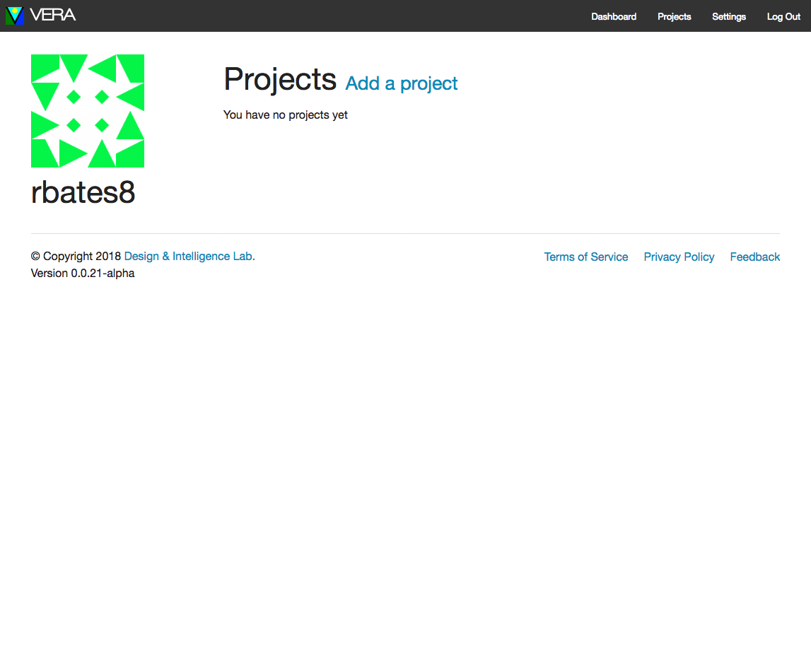
Initially there will be no projects, and you will need to click Add a project to create a new VERA project:

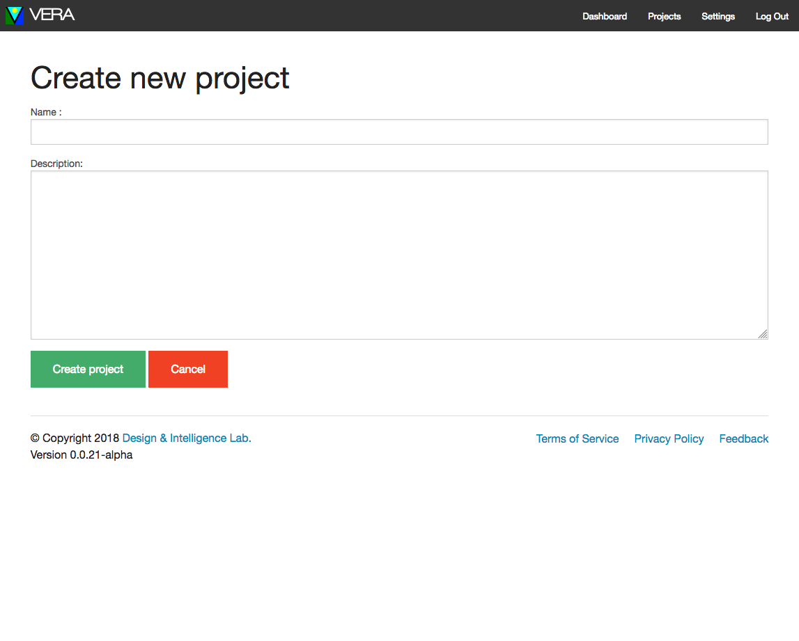
Give your project a brief name, and describe the phenomenon the project is exploring. In our case, let’s explore the food web of wolves, sheep, and grass and what happens if the system is unbalanced:

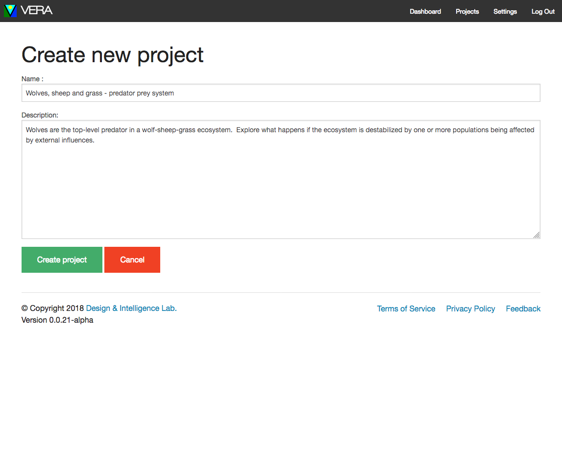
Click Create project to save your new project.

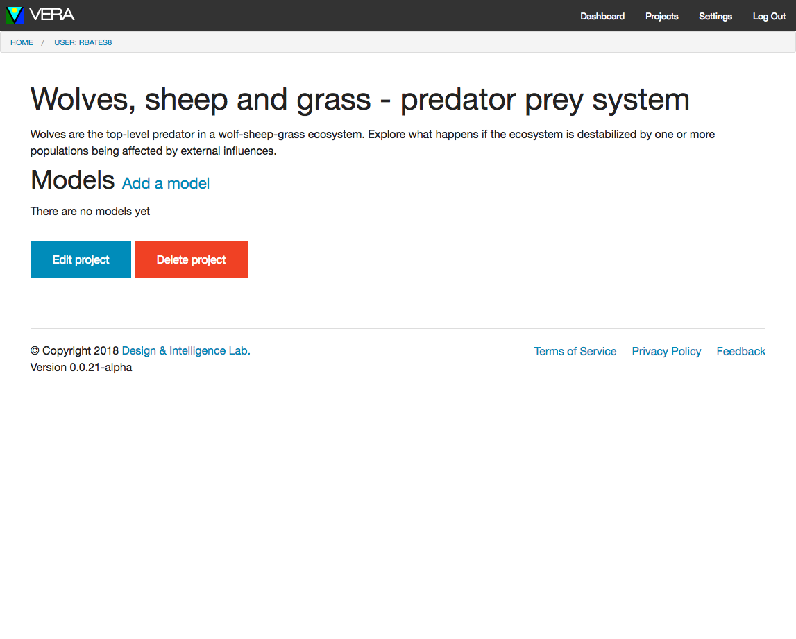
Great! We now have a new project, and now need to add one or more models to it.

Creating a model

In VERA, models are the basis for experimentation. With a model, you propose a hypothesis and then create a conceptual model to test the hypothesis. The model can be experimented with by executing the model as an agent-based simulation and observing the emergent behaviors of the agents, refining your model and re-running. This experimental feedback loop is the fundamental experimental workflow in VERA.

Creating a new model

On the project page, click the Add a model link to create a new model in this project:

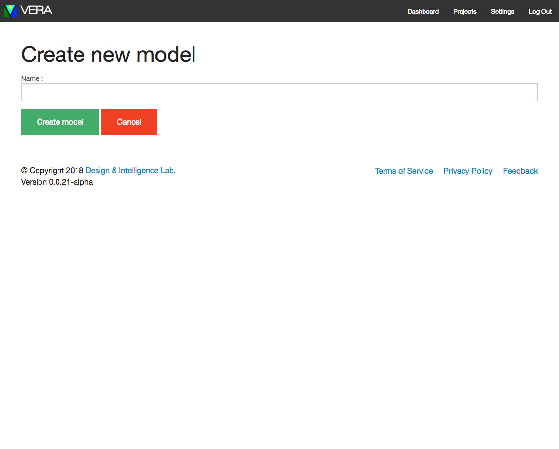
Let’s start off creating a new model that will be a base for further experimental models in this project, one that contains all the populations in the ecosystem in stable coexistence:

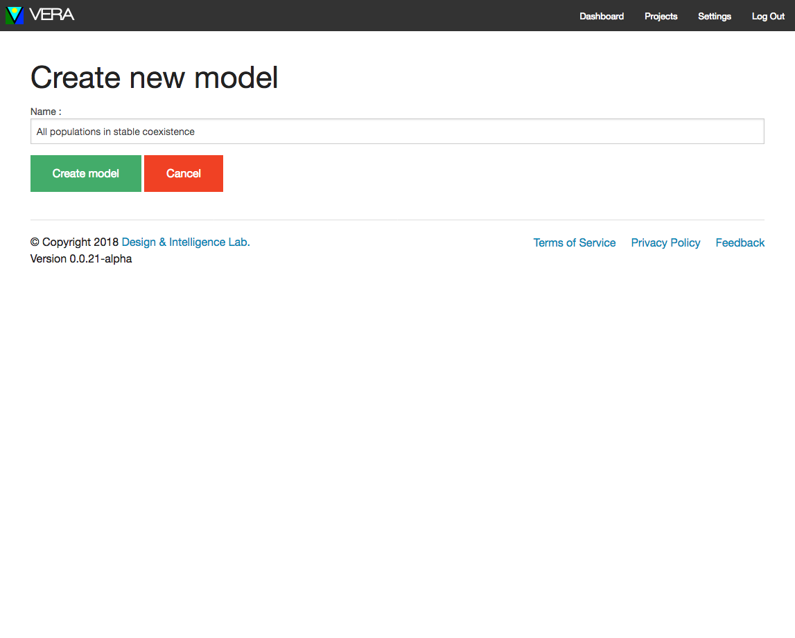
Clicking Create model will save a new empty model and open the model editor so you can begin building the conceptual model of your ecological system.

Getting to know the model editor

Now that we have created a model for our hypothesis and initialized a new model, we should see the following screen (minus the numbers in the editor regions, described below):

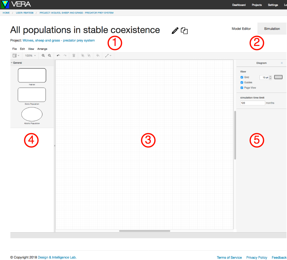
	This region of the model editor window displays the model name, containing project, and a link to the original model if this was cloned from another model. Edit the model name Clone the model to this project or another one
	The tabs Model and Simulation allow the user to toggle between the model editor and simulation panes, respectively.
	The center of the editor window is the model building workspace. This is where you will build your ecological model using Components and relationships, which we discuss in detail later.
	This left side panel is the Component panel, which contains model Components used to add biotic populations, habitats, and abiotic substances to the model.
	This right side panel is the modeling and simulation parameter editor. It is updated to reflect the currently selected Component or relationship in the model so aspects of both the conceptual model and simulation can be edited in one place. When no Component or relationship is selected, model-level properties are displayed here.

Managing Components

VERA currently supports the following Component types:

Component Type	Description
Biotic Population	A group of organisms to be modeled as a population with common parameters and behaviors
Abiotic Substance	Some non-biotic substance in the ecosystem being modeled that has an effect on other Biotic or Abiotic Components
Habitat	A region in the model that represents a distinct space where certain Biotic or Abiotic Substances can exist and interact

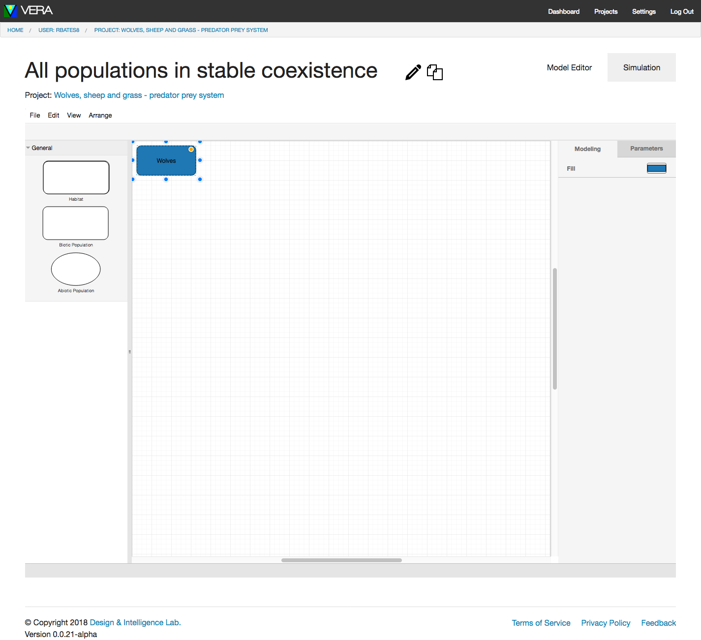
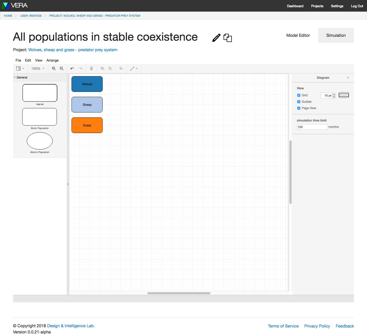
A good starter model is a simple ecosystem composed of wolves, sheep, and grass where we can study the impact of changes to each Component on the others. To start off, let’s add a new Component to the model. In the Component panel on the left, click on the Component labeled Biotic Population. You should see a new Component labeled “Biotic” added to your model:

You’ll notice that the right side properties editor now shows two tabs - one for Modeling and one for Parameters:

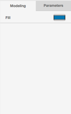
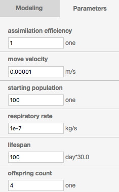
The Modeling tab will contain any settings for this Component related to the visual model. The Parameters tab contains parameters used for executing and tuning the simulation, which we will discuss in more detail later.

For now, we want to make this our Wolves population, so double-click the label and type in “Wolves” and hit the ENTER key on your keyboard:

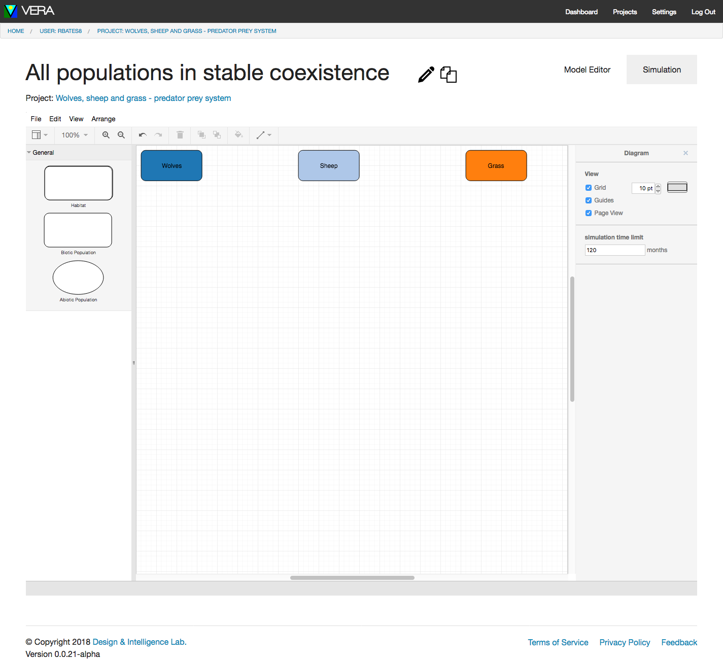
Now, let’s do the same thing for the Sheep and Grass populations. You should wind up with something like the following:

Now that we have some Biotic Components in the model for our populations, let’s move things around to give ourselves some more room to work with relationships in the next section. You can click on Components and drag-and-drop them to move them into different places to organize your model into a more coherent layout. Try moving your Sheep and Grass Components into the following layout:

Now that we have the major Components of our model in place, let’s investigate adding relationships between these Components to describe how they interact with each other.

Managing relationships

A relationship, as the name suggests, relates one Component to another in a directed manner (e.g. “Component X interacts with Component Y”). The allowed relationships will vary based on the source and destination Components selected, but will always be a subset of the Relations Ontology supported by EOL. The relationships implemented in VERA (where X is the source and Y is the destination for the directed relationship) are:

X destroys Y. When X interacts with Y, it partially or wholly destroys a simulation entity of type Y with no carbon transfer to X.
X produces Y: During the simulation, X will produce Y with some stochastic timing and amount.
X consumes Y. When X interacts with Y, it will partially or wholly consume Y, with carbon transfer to X from Y.
X becomes Y on death. When X expires, it produces Y.
X affects Y. This is a generic growth modifier that allows for growth rates (negative or positive) to modify Y when X interacts with it, where none of the above relationships apply.
X can migrate to Y. This relationship represents the ability of a Biotic or Abiotic Substance to move from its original Habitat to another Habitat in the model. It is created between a source Biotic or Abiotic Substance and a target Habitat. Without a Migrate relationship, Biotic and Abiotic Substance are constrained to the Habitat in which they are located.

To create a relationship between the Wolves and Sheep, hover your mouse cursor over the Wolves Component and you should see several small markers around the edge - these are relationship anchor points. Move your mouse cursor over one of those points and you will see a green halo around that marker. This indicates that you can create a relationship connection starting at this point to another Component in the model:

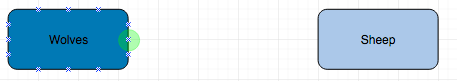
Click down on your left mouse button, hold it, and drag your mouse pointer to the Sheep Component (you should see the relationship stretching between the Wolves and your mouse pointer):

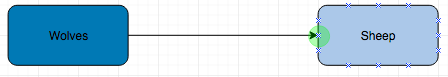
Once a green halo shows up on one of the Sheep Component’s relationship anchors, you can let go of the mouse button and you will now have a default Consumes relationship between these two populations: Wolves Consume Sheep.

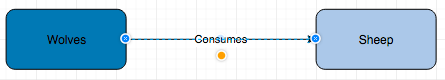
You can change the type of relationship by looking at the Modeling tab on the right side Properties panel and selecting a new type from the dropdown. Similar to Components, there is also a Parameters tab that will allow tuning of this relationship’s behavior in the simulation, which we will discuss later.

For now, let’s add another relationship to describe Sheep consuming Grass. You should wind up with something like the following (note the direction of the relationship arrows and make sure yours match!):

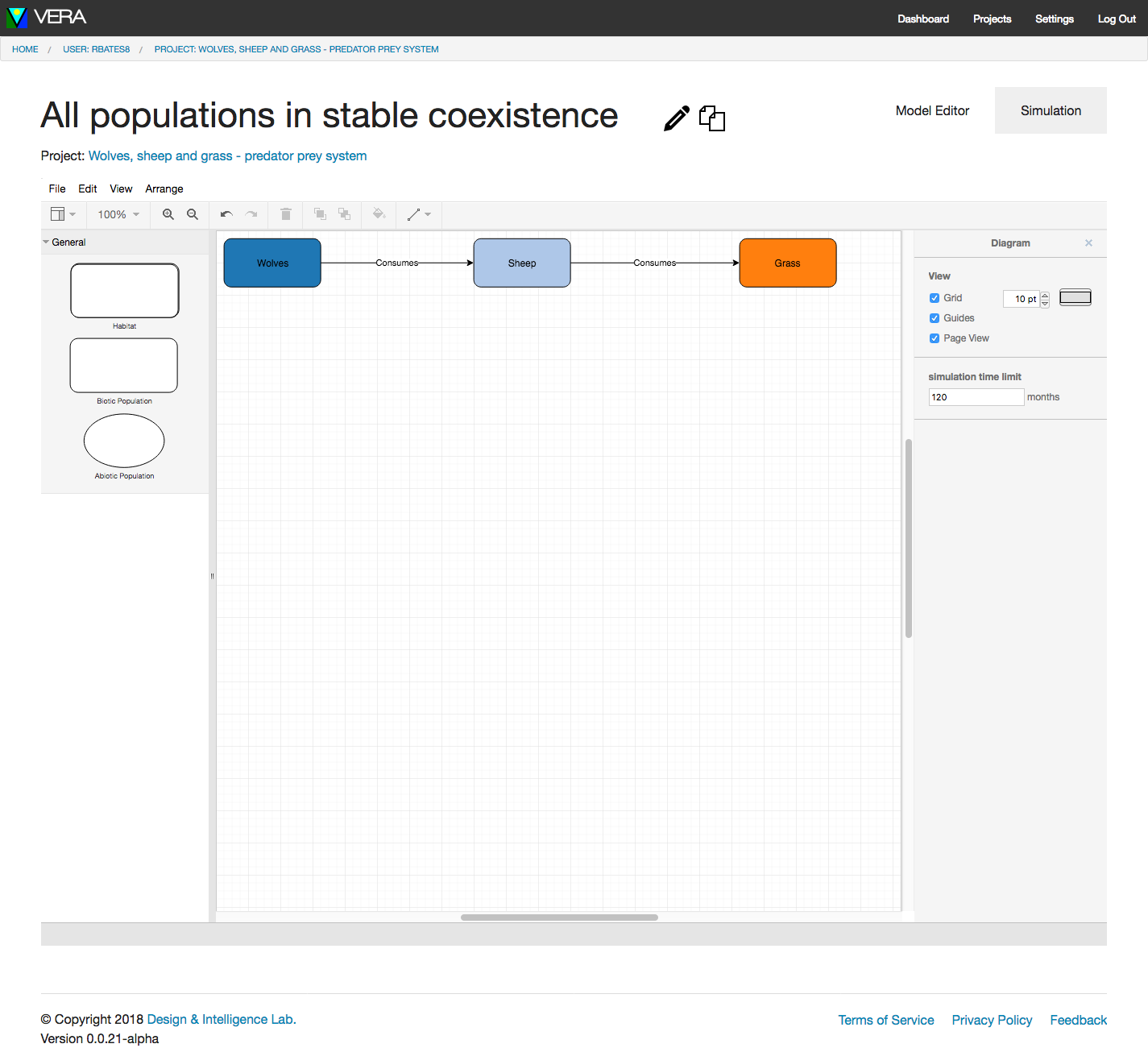
Congratulations! You have now built your first VERA model, and are ready to explore and refine it using the simulation feature of the system.

Simulating a model

A key feature of VERA is its ability to generate a simulation of the conceptual model we construct so we can validate (or invalidate) our hypothesis. In the case of the simple food web above, we can see how varying populations, lifespan, potential energy, etc. of populations can affect the organisms involved.

NOTE that simulations are artificially capped at 25,000 total agents to prevent "runaway" simulations from stalling and overextending the simulation engine. It is recommended to start out with smaller, localized populations rather than trying to model ecosystems on large scales until you have a better idea how your populations are going to interact with each other.

With our current model, let’s try running a simulation with the defaults and see what we get. To switch to the simulation, just click the Simulation tab in the upper right, and you should see a screen like this:

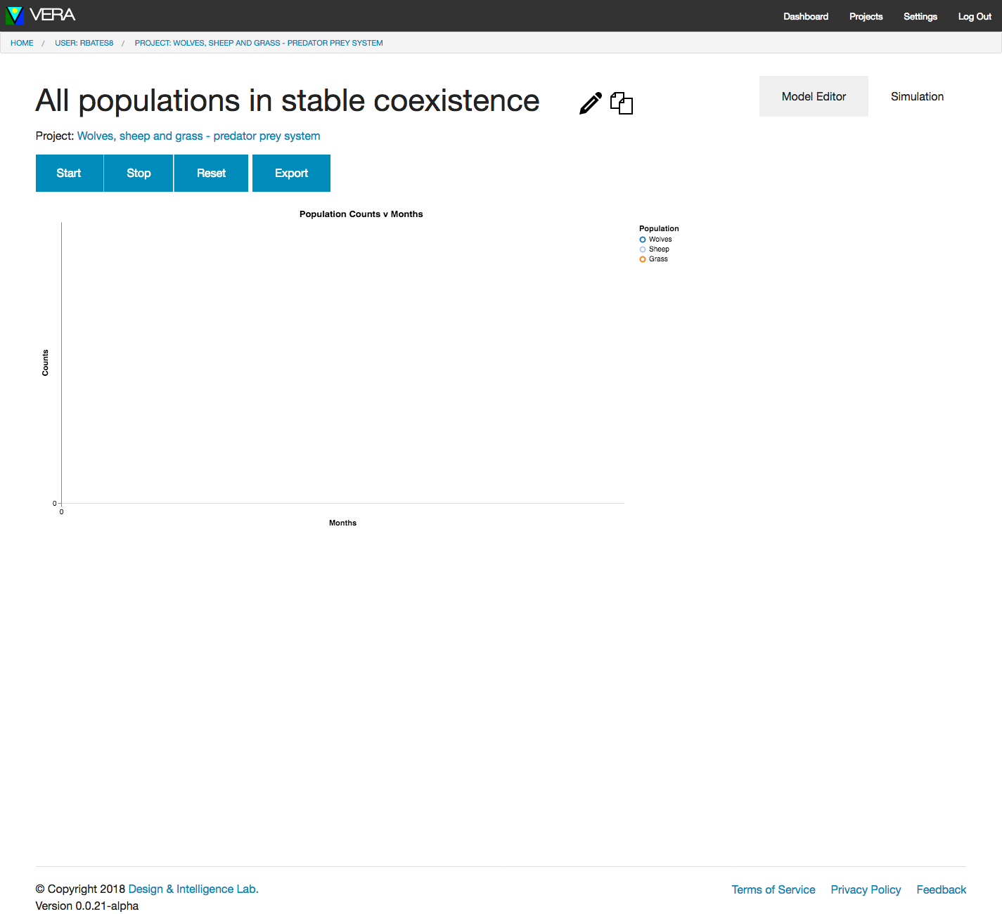
Start begins the simulation run.
Stop halts the simulation. You can start and stop a simulation as many times as you like until you hit the simulation time limit in months.
Reset clears the simulation and resets it to Day 1.
Export allows you to export the graph as a PNG image for download.

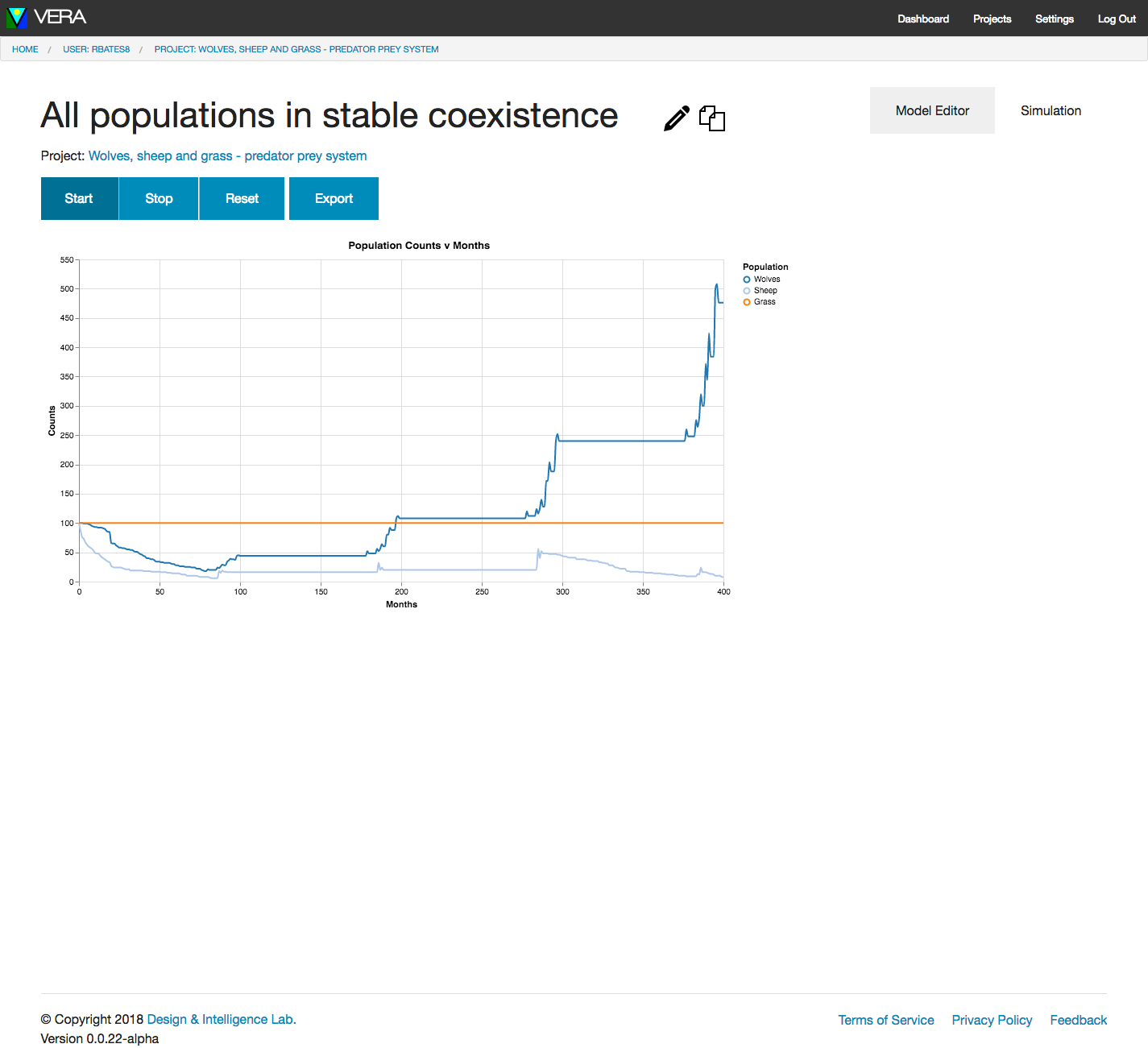
You should see a graph charting changes in populations over time, similar to below. The match may not be exact since there are some randomized elements to agent based simulations like this one.

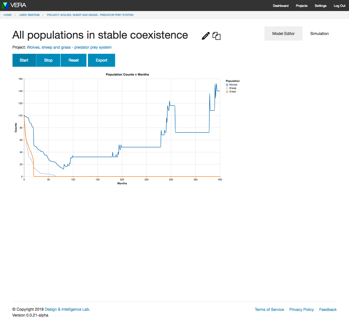
Right off the bat we can see that some things don’t look right:

Grass dies off almost immediately
Even though the Sheep population declines to zero, the Wolves continue to live - and actually in some cases increase in population.

This tells us we need to tune our model’s simulation parameters to more accurately reflect the actual populations and their behaviors.

Editing simulation parameters

To edit our model’s simulation parameters, just click on the Model Editor tab in the upper right of the page to return to the model editor. NOTE: Some browsers may recenter the model, so you might need to scroll your Components back into view when switching between the Model Editor and Simulation tabs.

Now that you are looking at the Wolves-Sheep-Grass model again, let’s make a few changes. For now, let’s assume that Grass is a perpetual population and never completely dies off. To make this change, click on the Grass Component and click the Parameters tab in the right properties panel:

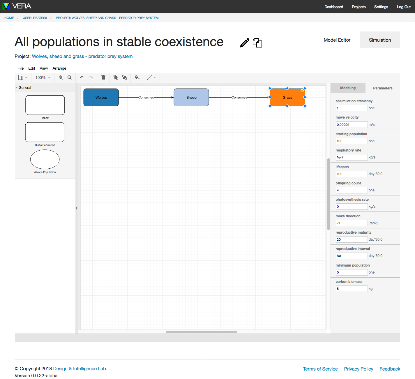
You will see a list of simulation parameters for the Grass population that you can tune to get the desired population behavior in the simulation. The following parameter values were partially supplied by the Smithsonian Institute’s Encyclopedia of Life (EOL) or discovered through experimentation with VERA. Change the following parameter values for the Grass population:

Parameter	New Value
move velocity	0
respiratory rate	0
lifespan	1
offspring count	0
photosynthesis rate	1
reproductive maturity	0
reproductive interval	0
minimum population	100

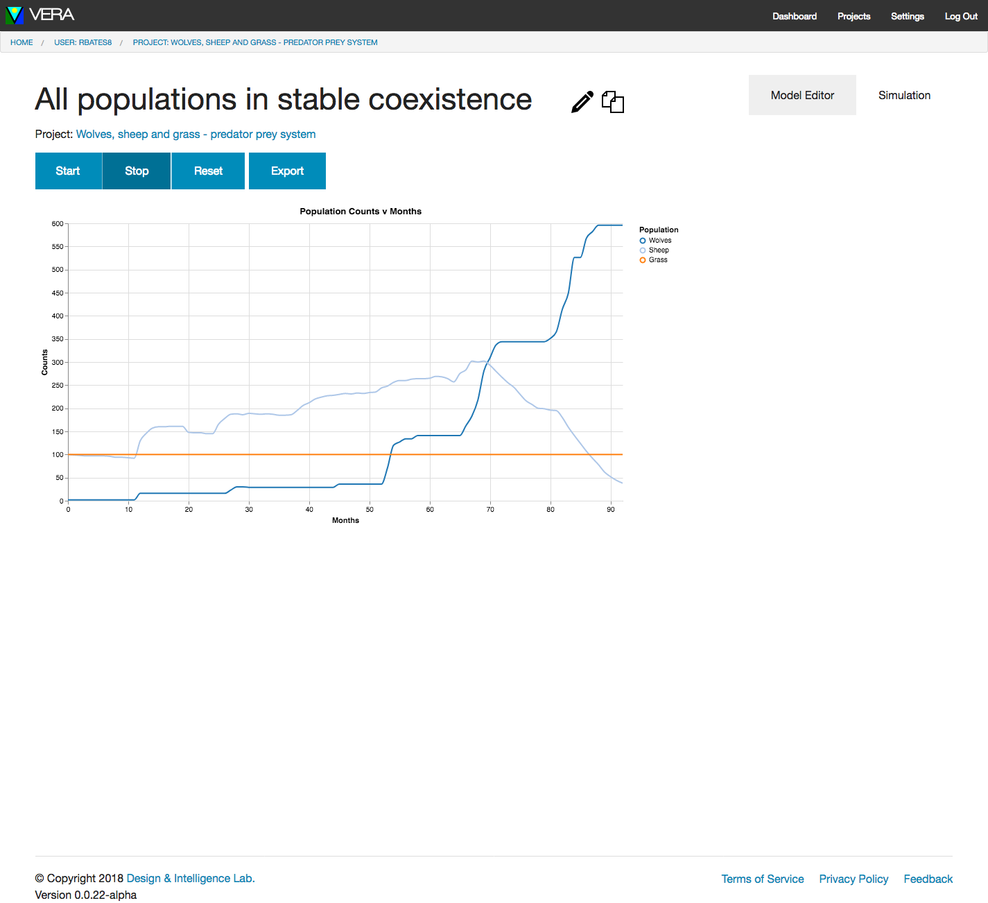
If you now click on the Simulation tab and rerun the simulation, you should see a stable Grass population, and the Sheep and Wolves populations start to cycle a bit closer to what you would expect:

However, we’re seeing an odd ratio of Wolves to Sheep; normally in such ecosystems there are actually fewer predators than prey in a ratio befitting the specific ecosystem. Not knowing exactly what this one should be, let’s try some things! Go back to the Model Editor and change the following Parameter values for the Wolves population:

Parameter	New Value
move velocity	0.035 (approx 3km/day)
starting population	2 (mating pair)
lifespan	180
offspring count	7
reproductive maturity	30
reproductive interval	12

Also change several of the Parameters for the Sheep population by selecting the Sheep Component and specifying these values:

Parameter	New Value
move velocity	0.01 (approx 1km/day)
lifespan	235
offspring count	1
reproductive maturity	42
reproductive interval	12

Running the simulation with the new parameters should give you something more expected: as the number of predators increases, the number of prey decrease, and the populations fall into a predator-prey/boom-bust cycle (your graph might differ slightly due to randomness introduced in the simulation):

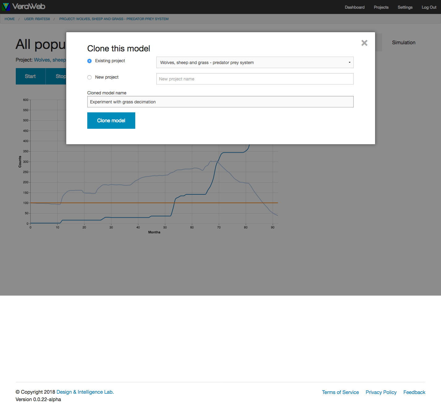
Play with the parameters on the relationships as well to see how they affect the simulation. Once you have a model that exhibits your ecosystem’s baseline behavior, clone it (using the icon next to the model name at the top of the page) to a new model so you can experiment with the new model and not lose your original:

Personalized Learning Coaches

The personalized learning coaches provide feedback based on your modeling behaviors and the model itself. They guide you through an exploratory process to help you better reason your model by formulating hypotheses, experimentally evaluating them, and reflecting on the outcomes. After viewing the feedback, you will need to exit out of the feedback window to perform the suggested actions. Clicking on the button again would return the same feedback if you saved it. When you are done interacting with the feedback and have written responses in the fields, click "Submit” so the coach can provide new feedback the next time you interact with it.

Exploration Coach

The aim for the exploration coach is to help you conduct the process of constructing models, changing parameters in models, and simulating models. The coach gives adaptive feedback based on your modeling behavior, and it may suggest actions such as creating a new component in your model or changing a set of parameters. Each set of feedback comes with reflective questions for you to answer.

Recommendation Coach

The aim for the recommendation coach is to provide a similar model to the one you are working on, so that you can explore how its components interact and make connections about how similar changes would affect your own model. The first step the coach will ask you to take is cloning the recommended model. This will open a new tab with the model in it. From there, it will provide general guidance on how to explore the model, reason about the behaviors you observe, and ask you to perform reflection on the results and how they may relate to your own model.

Getting Help

We hope that this user guide has provided you with the information needed to get started with VERA. If you do find you need assistance, the recommended way is to click the Feedback link in the web page footer and fill out the form:

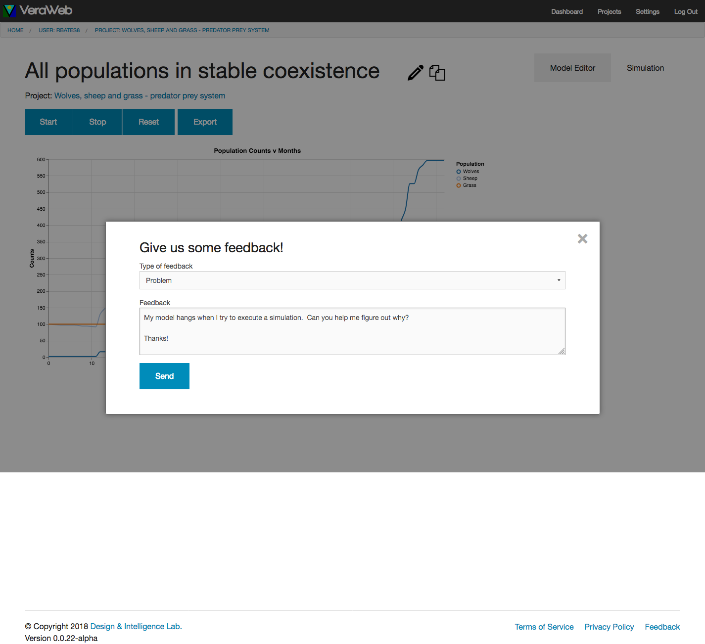
We are immediately notified of the feedback, and it is logged in our tracking system. If however the website is not processing th feedback form, or you require some other assistance, please email us at veraweb@cc.gatech.edu and someone from the team will reply as quickly as possible. If you do choose to email us regarding a technical issue, please provide us with the following information along with your issue:

Operating system (type and version, e.g. macOS 10.13.6)
Browser and version (e.g. Google Chrome, Version 68.0.3440.106)
If possible, the address of the web page you were experiencing problems on, copied from the address bar in your browser.

Thanks for using VERA!

References

Goel, A. K., Rugaber, S., Joyner, D. A., Vattam, S., Hmelo-Silver, C., Jordan, R., Sinha, S., Honwad, S., & Eberbach, C. (2013). Learning Functional Models of Aquaria: The ACT Project on Ecosystem Learning in Middle School Science. International Handbook of Metacognition and Learning Technologies, R. Azevedo & V. Aleven (editors). Springer International Handbooks of Education Volume 28, 2013, pp 545-559.

Goel, A. K., Vattam, S., Rugaber, S., Joyner, D. A., Hmelo-Silver, C., Jordan, R., Honwad, S., Gray, S., & Sinha, S. (2010). Learning Functional and Causal Abstractions of Classroom Aquaria. In Proceedings of the 32nd Annual Meeting of the Cognitive Science Society, Portland, Oregon.

Joyner, D. A., Goel, A. K., & Papin, N. (2014). MILA-S: Generation of agent-based simulations from conceptual models . In Proceedings of the 19th International Conference on Intelligent User Interfaces. Haifa, Israel. pp. 289-298.

Joyner, D. A., Goel, A. K., & Majerich, D. (2013). Metacognitive Tutoring for Scientific Modeling. AIED 2013 Workshops Proceedings Scaffolding in Open-Ended Learning Environments (OELEs)

Wilensky, U. (1999). NetLogo. http://ccl.northwestern.edu/netlogo/. Center for Connected Learning and Computer-Based Modeling, Northwestern University, Evanston, IL.

Appendix A: Simulation Parameters

Biotic Population

A Biotic Population is used to model a population of living organisms. Some of the parameters below are aggregate for the entire population, some are averages to be used when manipulating individual organisms within the population. The descriptions should differentiate between the two.

Parameter	Units	Description
assimilation efficiency	one	When one thing consumes another, not all the carbon is assimilated by the consumer – some is burned off, some is passed as waste. This parameter is the percentage of carbon biomass retained by the consumer. Say the rate is 0.90, if they consume something that has 1kg of carbon biomass, 0.9kg is added to the consumer and 0.1kg is “lost” to the environment.
move velocity	m/s	Average velocity of the organisms in this population as they move in their environment.
starting population	one	Starting population size for this Component.
respiratory rate	kg/s	Resting metabolic rate measured in loss of carbon biomass so we can model starvation/dissipation.
lifespan	day*30.0	Average lifespan of this species in months^[a].
offspring count	one	Average number of offsprings birthed/spawned at a time.
photosynthesis rate	kg/s	This is the rate at which photosynthetic organisms can add carbon biomass to themselves.
move direction	[rad?]^[b]^[c]	General direction the population moves, in degrees heading where North is 0, East is 90, South is 180, and West is 270. This can be used to study migrations, flows, etc.
reproductive maturity	day*30.0	The age at which a biotic organism is able to begin reproducing; related to “reproductive interval” which controls how often the population’s organisms can reproduce after they reach the age of reproductive maturity.
reproductive interval	day*30.0	How frequently individuals in the population can reproduce once they have reached reproductive maturity.
minimum population	one	For perpetual populations, this sets the minimum size of the population that the system tries to maintain.
carbon biomass	kg	This is the amount of carbon in a typical adult organism from a biotic population. It is the analogue for energy flow in the ecosystem since research typically doesn’t measure energy (e.g. joules, watts, etc) but does and can measure the change in carbon mass of organisms.

Abiotic Substance

An Abiotic Substance is currently used to represent some quantity of a non-living substance in the model that interacts with Biotic and Abiotic Substances.

Parameter	Units	Description
amount	kg	Starting amount of the abiotic substance per grid location in the simulation environment.
minimum amount	kg	For perpetual populations, this sets the minimum size of the population that the system tries to maintain.
growth rate	%	Allows this population to grow (positive rate) or shrink (negative rate) as the simulation executes, regardless of interactions with other Components in the system.

Habitat

The Habitat Component is intended to encapsulate microenvironments where populations can interact with each other. Populations can flow between Habitats where defined, but are otherwise constrained to the Habitat they are defined in.

Parameter	Units	Description
drift velocity	m/s	Velocity added to agents within populations contained in this Habitat. This could represent a slope, current (water or air), or some other environmental force that would affect the movement of agents.
drift direction	[rad?]	General direction the populations in this Habitat will move, in degrees heading where North is 0, East is 90, South is 180, and West is 270.